5. Two-Dimensional Solver
5.1. Dimensional Splitting
In this assignment, we’ll enhance our wavepropagation to handle two-dimensional problems by implementing Dimensional Splitting. This approach eliminates the need to modify our fwave solver; instead, we’ll perform separate x-sweeps and y-sweeps on the grid using these function:
x-sweep:
y-sweep:
We need to transition from wavepropagation1d to wavepropagation2d.
There are various approaches to tackle the problem:
Using a 3D array to store the grid and accessing all elements through it, where the first dimension is dedicated to storing the steps, and the other two dimensions represent the x and y coordinates..
Employing a 2D array with a quadratic number of cells, where the first dimension represents the steps, and the second dimension corresponds to the x and y coordinates. Specific cells are accessed using a designated formula.
t_idx l_id = l_iy * i_stride + l_ix;
and we will use the second approach.
Now, we will need to create three files. :
WavePropagation2d.h,WavePropagation2d.cppandWavePropagation2d.test.cpp:2.1. Let’s begin with our
WavePropagation2d.h. OurWavePropagation2d.hwill resemble the 1D version but with some modifications to the following functions:private : tsunami_lab::t_idx getIndex(tsunami_lab::t_idx i_ix,tsunami_lab::t_idx i_iy){ return (m_nCells+2) * i_iy +i_ix; } public: void setHeight( t_idx i_ix, t_idx i_iy, t_real i_h ) { m_h[m_step][getIndex(i_ix+1,i_iy+1)] = i_h; } void setBathymetry(t_idx i_ix, t_idx i_iy, t_real i_b){ m_b[getIndex(i_ix+1,i_iy+1)] = i_b; } void setMomentumX( t_idx i_ix, t_idx i_iy, t_real i_hu ) { m_hu[m_step][getIndex(i_ix+1,i_iy+1)] = i_hu; } void setMomentumY( t_idx i_ix, t_idx i_iy, t_real i_hv) { m_hv[m_step][getIndex(i_ix+1,i_iy+1)] = i_hv; }
2.2. now lest start implementing
wavepropagation2d.cpp. OurWavePropagation2d.cppwill resemble the 1D version but with some modifications to the following functions:tsunami_lab::patches::WavePropagation2d::WavePropagation2d( t_idx i_nCells, bool i_choice ) { m_choice = i_choice; m_nCells = i_nCells; // allocate memory including a single ghost cell on each side for( unsigned short l_st = 0; l_st < 2; l_st++ ) { m_h[l_st] = new t_real[ (m_nCells+2) * (m_nCells+2) ]; m_hu[l_st] = new t_real[ (m_nCells+2) * (m_nCells+2) ]; m_hv[l_st] = new t_real[ (m_nCells+2) * (m_nCells+2) ]; } m_b = new t_real[(m_nCells+2) * (m_nCells+2)]; // init to zero for( unsigned short l_st = 0; l_st < 2; l_st++ ) { for( t_idx l_ce = 0; l_ce < (m_nCells+2) * (m_nCells+2) ; l_ce++ ) { m_h[l_st][l_ce] = 0; m_hu[l_st][l_ce] = 0; m_hv[l_st][l_ce] = 0; m_b[l_ce] = 0; } } } //free memory tsunami_lab::patches::WavePropagation2d::~WavePropagation2d() { for( unsigned short l_st = 0; l_st < 2; l_st++ ) { delete[] m_h[l_st]; delete[] m_hu[l_st]; delete[] m_hv[l_st]; } delete[] m_b; }
Now, let’s implement the x-sweep and y-sweep in the “
wavepropagation2d.cppvoid tsunami_lab::patches::WavePropagation2d::timeStep( t_real i_scaling) { // pointers to old and new data t_real * l_hOld = m_h[m_step]; t_real * l_huOld = m_hu[m_step]; t_real * l_hvOld = m_hv[m_step]; t_real * l_b = m_b; m_step = (m_step+1) % 2; _real * l_hNew = m_h[m_step]; t_real * l_huNew = m_hu[m_step]; t_real * l_hvNew = m_hv[m_step]; for( t_idx l_ce = 1; l_ce < ((m_nCells+2) * (m_nCells+2)); l_ce++ ) { l_hNew[l_ce] = l_hOld[l_ce]; l_huNew[l_ce] = l_huOld[l_ce]; l_hvNew[l_ce] = l_hvOld[l_ce]; } setGhostOutflow(true); //x-sweep for(t_idx l_ex = 0; l_ex < m_nCells +1;l_ex++){ for(t_idx l_ey = 0; l_ey < m_nCells +1;l_ey++){ t_real l_netUpdates[2][2]; t_idx l_ceL = getIndex(l_ey,l_ex); t_idx l_ceR = getIndex(l_ey+1,l_ex); if(m_choice){ solvers::Roe::netUpdates(l_hOld[l_ceL], l_hOld[l_ceR], l_huOld[l_ceL], l_huOld[l_ceR], l_netUpdates[0], l_netUpdates[1]); }else{ solvers::fwave::netUpdates( l_hOld[l_ceL], l_hOld[l_ceR], l_huOld[l_ceL], l_huOld[l_ceR], l_b[l_ceL], l_b[l_ceR], l_netUpdates[0], l_netUpdates[1]); } l_hNew[l_ceL] -= i_scaling * l_netUpdates[0][0]; l_huNew[l_ceL] -= i_scaling * l_netUpdates[0][1]; l_hNew[l_ceR] -= i_scaling * l_netUpdates[1][0]; l_huNew[l_ceR] -= i_scaling * l_netUpdates[1][1]; } } l_hOld = m_h[m_step]; l_huOld = m_hu[m_step]; l_hvOld = m_hv[m_step]; m_step = (m_step+1) % 2; l_hNew = m_h[m_step]; l_huNew = m_hu[m_step]; l_hvNew = m_hv[m_step]; for( t_idx l_ce = 1; l_ce < ((m_nCells+2) * (m_nCells+2)); l_ce++ ) { l_hNew[l_ce] = l_hOld[l_ce]; l_huNew[l_ce] = l_huOld[l_ce]; l_hvNew[l_ce] = l_hvOld[l_ce]; } setGhostOutflow(true); //y-sweep for(t_idx l_ex = 0; l_ex < m_nCells +1;l_ex++){ for(t_idx l_ey = 0; l_ey < m_nCells +1;l_ey++){ t_real l_netUpdates[2][2]; t_idx l_ceL = getIndex(l_ey,l_ex); t_idx l_ceR = getIndex(l_ey,l_ex+1); if(m_choice){ solvers::Roe::netUpdates( l_hOld[l_ceL], l_hOld[l_ceR], l_hvOld[l_ceL], l_hvOld[l_ceR], l_netUpdates[0], l_netUpdates[1]); }else{ solvers::fwave::netUpdates( l_hOld[l_ceL], l_hOld[l_ceR], l_hvOld[l_ceL], l_hvOld[l_ceR], l_b[l_ceL], l_b[l_ceR], l_netUpdates[0], l_netUpdates[1]); } l_hNew[l_ceL] -= i_scaling * l_netUpdates[0][0]; l_hvNew[l_ceL] -= i_scaling * l_netUpdates[0][1]; l_hNew[l_ceR] -= i_scaling * l_netUpdates[1][0]; l_hvNew[l_ceR] -= i_scaling * l_netUpdates[1][1]; } } }
Let’s implement our boundary:
void tsunami_lab::patches::WavePropagation2d::setGhostOutflow(bool i_choiceBoundry) {
    m_choiceBoundry = i_choiceBoundry;
    t_real * l_h = m_h[m_step];
    t_real * l_hu = m_hu[m_step];
    t_real * l_hv = m_hv[m_step];
    t_real * l_b = m_b;
    for (unsigned short l_qw = 0; l_qw < 2; ++l_qw){
        for (unsigned short l_qe = 0; l_qe < 2; ++l_qe){
            const int i = l_qw * (m_nCells + 2);
            const int j = l_qe * (m_nCells + 2);
            const int targetIndex = (m_nCells + 2 - l_qw) * (m_nCells + 2) + l_qe;

            l_h[targetIndex] = l_h[i + j + l_qe + 1];
            if(i_choiceBoundry){
            l_hu[targetIndex] = -l_hu[i + j + l_qe + 1];
            l_hv[targetIndex] = -l_hv[i + j + l_qe + 1];
            }
            else
            {
                l_hu[targetIndex] = l_hu[i + j + l_qe + 1];
                l_hv[targetIndex] = l_hv[i + j + l_qe + 1];
            }
            l_b[targetIndex] = l_b[i + j + l_qe + 1];
        }
    }
    // bottom row & top row
    for (t_idx l_g = 1; l_g < m_nCells; l_g++)
    {
        l_h[l_g] = l_h[getIndex(l_g,1)];
        l_h[getIndex(l_g,m_nCells+1)] = l_h[getIndex(l_g,m_nCells)];

        if(i_choiceBoundry)
        {
            l_hu[l_g] = -l_hu[getIndex(l_g,1)];
            l_hu[getIndex(l_g,m_nCells+1)] = -l_hu[getIndex(l_g,m_nCells)];
            l_hv[l_g] = -l_hv[getIndex(l_g,1)];
            l_hv[getIndex(l_g,m_nCells+1)] = -l_hv[getIndex(l_g,m_nCells)];
        }
        else
        {
            l_hu[l_g] = l_hu[getIndex(l_g,1)];
            l_hu[getIndex(l_g,m_nCells+1)] = l_hu[getIndex(l_g,m_nCells)];
            l_hv[l_g] = l_hv[getIndex(l_g,1)];
            l_hv[getIndex(l_g,m_nCells+1)] = l_hv[getIndex(l_g,m_nCells)];
        }
        l_b[l_g] = l_b[getIndex(l_g,1)];
        l_b[getIndex(l_g,m_nCells+1)] = l_b[getIndex(l_g,m_nCells)];
    }

    // leftest and rightest column
    for (t_idx l_g = 1; l_g < m_nCells; l_g++)
    {
        l_h[getIndex(0,l_g)] = l_h[getIndex(1,l_g)];
        l_h[getIndex(m_nCells+1,l_g)] = l_h[getIndex(m_nCells,l_g)];
        if(i_choiceBoundry)
        {
            l_hu[getIndex(0,l_g)] = -l_hu[getIndex(1,l_g)];
            l_hu[getIndex(m_nCells+1,l_g)] = -l_hu[getIndex(m_nCells,l_g)];
            l_hv[getIndex(0,l_g)] = -l_hv[getIndex(1,l_g)];
            l_hv[getIndex(m_nCells+1,l_g)] = -l_hv[getIndex(m_nCells,l_g)];
        }
        else
        {
            l_hu[getIndex(0,l_g)] = l_hu[getIndex(1,l_g)];
            l_hu[getIndex(m_nCells+1,l_g)] = l_hu[getIndex(m_nCells,l_g)];
            l_hv[getIndex(0,l_g)] = l_hv[getIndex(1,l_g)];
            l_hv[getIndex(m_nCells+1,l_g)] = l_hv[getIndex(m_nCells,l_g)];
        }
            l_b[getIndex(0,l_g)] = l_b[getIndex(1,l_g)];
            l_b[getIndex(m_nCells+1,l_g)] = l_b[getIndex(m_nCells,l_g)];
    }

            // Ecken des Gitters aktualisieren
                          //[0/0]
            l_b[getIndex(0,0)] = l_b[getIndex(1,1)];
            l_b[getIndex(m_nCells+1,0)] = l_b[getIndex(m_nCells,1)];
            l_b[getIndex(0,m_nCells+1)] = l_b[getIndex(1,m_nCells)];
            l_b[getIndex(m_nCells+1,m_nCells+1)] = l_b[getIndex(m_nCells,m_nCells)];

            l_h[getIndex(0,0)] = l_h[getIndex(1,1)];
            l_h[getIndex(m_nCells+1,0)] = l_h[getIndex(m_nCells,1)];
            l_h[getIndex(0,mopo_nCells+1)] = l_h[getIndex(1,m_nCells)];
            l_h[getIndex(m_nCells+1,m_nCells+1)] = l_h[getIndex(m_nCells,m_nCells)];

            l_hu[getIndex(0,0)] = l_hu[getIndex(1,1)];
            l_hu[getIndex(m_nCells+1,0)] = l_hu[getIndex(m_nCells,1)];
            l_hu[getIndex(0,m_nCells+1)] = l_hu[getIndex(1,m_nCells)];
            l_hu[getIndex(m_nCells+1,m_nCells+1)] = l_hu[getIndex(m_nCells,m_nCells)];

            l_hv[getIndex(0,0)] = l_hv[getIndex(1,1)];
            l_hv[getIndex(m_nCells+1,0)] = l_hv[getIndex(m_nCells,1)];
            l_hv[getIndex(0,m_nCells+1)] = l_hv[getIndex(1,m_nCells)];
            l_hv[getIndex(m_nCells+1,m_nCells+1)] = l_hv[getIndex(m_nCells,m_nCells)];
     }
}
Important
tsunami_lab::t_idx getIndex(tsunami_lab::t_idx i_ix,tsunami_lab::t_idx i_iy){ return (m_nCells+2) * i_iy +i_ix; }
where our strid is m_nCells+2
finally lets implement the
WavePropagation2d.test.cpp:#include <catch2/catch.hpp> #include "WavePropagation2d.h" TEST_CASE( "Test the 2d wave propagation solver.", "[WaveProp2d]" ) { tsunami_lab::patches::WavePropagation2d m_waveProp( 100 , true ); std::size_t l_ce; for( std::size_t l_ce = 0; l_ce < 100+1; l_ce++ ) { for( std::size_t l_cy = 0; l_cy < 100+1; l_cy++ ){ m_waveProp.setHeight( l_ce, l_cy, 5 ); m_waveProp.setMomentumX( l_ce, l_cy, 0 ); m_waveProp.setMomentumY( l_ce, l_cy, 0 ); m_waveProp.setGhostOutflow(true); } } // set outflow boundary condition // perform a time step m_waveProp.setGhostOutflow(true); m_waveProp.timeStep(0.1); // steady state for( std::size_t l_cy = 1; l_cy < 50 ; l_cy++ ) { for( std::size_t l_cx = 1; l_cx < 100 ; l_cx++ ) { l_ce = (l_cx+1) + (l_cy+1 ) * (100+2); REQUIRE( m_waveProp.getHeight()[l_ce] == Approx( 5.0f) ); REQUIRE( m_waveProp.getMomentumX()[l_ce] == Approx( 0 ) ); } } REQUIRE( m_waveProp.getHeight()[49] == Approx(5.0) ); REQUIRE( m_waveProp.getMomentumX()[49] == Approx( 0.0 )); REQUIRE( m_waveProp.getHeight()[50] == Approx(5.0) ); REQUIRE( m_waveProp.getMomentumX()[50] == Approx(0.0) ); // steady state for( std::size_t l_ce = 50; l_ce < 100; l_ce++ ) { REQUIRE( m_waveProp.getHeight()[l_ce] == Approx(5.0) ); REQUIRE( m_waveProp.getMomentumX()[l_ce] == Approx(0.0) ); } }
5.1.1. circular dam break setup
After enabling our wavepropagation to accommodate a 2D system, we can now proceed to implement a circular dam break setup within the specified domain \([-50, 50]^2\) This will be achieved by utilizing the following initial values:
\[\begin{split}\begin{cases} [h, hu, hv]^T = [10, 0, 0]^T &\text{if } \sqrt{x^2+y^2} < 10 \\ [h, hu, hv]^T = [5, 0, 0]^T \quad &\text{else} \end{cases}\end{split}\]
We need to generate the following files in setup: DamBreak2d.cpp , DamBreak2d.h and DamBreak2d.test.cpp
lets start by implemeting
DamBreak2d.h
#ifndef TSUNAMI_LAB_SETUPS_DAM_BREAK_2D_H
#define TSUNAMI_LAB_SETUPS_DAM_BREAK_2D_H

#include "../Setup.h"

namespace tsunami_lab {
  namespace setups {
    class DamBreak2d;
  }
}

/**
* 2d dam break setup.
**/
class tsunami_lab::setups::DamBreak2d: public Setup {

public:

  /**
   * @brief Gets the water height at a given point.
   *
   * @param i_x x-coordinate of the queried point.
   * @return height at the given point.
   **/
  t_real getHeight( t_real i_x,
                    t_real i_y) const;

  /**
   * @brief Gets the momentum in x-direction.
   *
   * @return momentum in x-direction.
   **/
  t_real getMomentumX( t_real,
                       t_real ) const;

  /**
   * @brief Gets the momentum in y-direction.
   * @return momentum in y-direction.
   **/
  t_real getMomentumY( t_real,
                       t_real ) const;

  /**
   * @brief Gets the bathymetry.
   * @return bathymetry.
   **/
  t_real getBathymetry( t_real,
                        t_real ) const ;
};

#endif
lets implement the
DamBreak2d.cpp:
#include "DamBreak2d.h"
#include "cmath"

tsunami_lab::t_real tsunami_lab::setups::DamBreak2d::getHeight( t_real i_x,
                                                            t_real i_y) const {
  if(std::sqrt((i_x*i_x)+(i_y*i_y)) < 10){
    return 10;
  } else{
    return 5;
  }

}

tsunami_lab::t_real tsunami_lab::setups::DamBreak2d::getMomentumX( t_real ,
                                                               t_real ) const {
  return 0;
}


tsunami_lab::t_real tsunami_lab::setups::DamBreak2d::getMomentumY( t_real ,
                                                               t_real ) const {
  return 0;
}

tsunami_lab::t_real tsunami_lab::setups::DamBreak2d::getBathymetry( t_real ,
                                                                t_real ) const {
  return 0;
}
now lets implement our test unit for the circular dambreak in the
DamBreak2d.test.cpp:
#include <catch2/catch.hpp>
#include "DamBreak2d.h"

TEST_CASE( "Test the two-dimensional dam break setup.", "[DamBreak2d]" ) {
  tsunami_lab::setups::DamBreak2d l_damBreak;

  // left side
  REQUIRE( l_damBreak.getHeight( 2, 4 ) == 10.0 );

  REQUIRE( l_damBreak.getMomentumX( 2, 0 ) == 0 );

  REQUIRE( l_damBreak.getMomentumY( 2, 0 ) == 0 );

  REQUIRE( l_damBreak.getHeight( 2, 5 ) == 10.0  );

  REQUIRE( l_damBreak.getMomentumX( 2, 5 ) == 0 );

  REQUIRE( l_damBreak.getMomentumY( 2, 2 ) == 0 );

  // right side
  REQUIRE( l_damBreak.getHeight( 4, 0 ) == 10.0  );

  REQUIRE( l_damBreak.getMomentumX( 4, 0 ) == 0 );

  REQUIRE( l_damBreak.getMomentumY( 4, 0 ) == 0 );

  REQUIRE( l_damBreak.getHeight( 4, 5 ) == 10.0  );

  REQUIRE( l_damBreak.getMomentumX( 4, 5 ) == 0 );

  REQUIRE( l_damBreak.getMomentumY( 4, 2 ) == 0 );
}
simulation
Now, we’ll model the circular DamBreak, incorporating a reflective boundary.
In the simulation, we will observe how the waves reflect on the border of our domain.
5.1.2. Illustration of the support for bathymetry
Include bathymetric data in our circular DamBreak simulation:
First, let’s modify our ‘getBathymetry’ function:
tsunami_lab::t_real tsunami_lab::setups::DamBreak2d::getBathymetry( t_real i_x,
                                                                  t_real ) const {
if( (i_x > 35) &  (i_x < 40) ){
  return 10 ;
}else{
  return 0;
  }
}
And don’t forget to set the water height to zero wherever the bathymetry is present
tsunami_lab::t_real tsunami_lab::setups::DamBreak2d::getHeight( t_real i_x,
                                                              t_real i_y) const {

  if( (i_x > 35) &  (i_x < 40) ){
    return 0 ;
  }else{

    if(std::sqrt((i_x*i_x)+(i_y*i_y)) < 10){
      return 10;
    } else{
      return 5;
    }
  }

}
In the simulation, we’ll observe how water waves interact and reflect off the obstacle we’ve introduced.
5.2. Stations
5.2.1. Add a new class Stations
There are numerous methods for implementing a station class, but we chose to implement it using a struct object for the station. Initially, we create a struct object for the station and include it in the constant.h file.
struct Station {
  std::string i_name;
  tsunami_lab::t_real i_x,i_y;
  };
To retrieve user data for the station, we first created a JSON file named stations.json in the configs folder.
{
    "frequency": 2,
    "stations": [
        {
            "i_name": "Dart",
            "i_x": -51,
            "i_y": -51
        },
        {
            "i_name": "Habibi",
            "i_x": 0.75,
            "i_y": 30.75
        }
    ]
}
Important
You have the option to include station data in the JSON file, and upon running
the code, the stations will be automatically written to the station folder.
The station’s coordinates must fall within our designated boundary, in our case within the range of \([-50, 50]^2\). If the coordinates lie outside this boundary, they will not be saved in the station folder.
the boundary can be effected throguh the following inputs (dimension domain_start) thats can be found in the config.json file.
Now, we need to create functions in the \tsunami_lab\src\io\JsReader\Configuration.cpp file to read data from a JSON file and . One function should be implemented
to retrieve the coordinates of the stations, and another one to retrieve the frequency.
  void tsunami_lab::io::Configuration::readStationsFromJson(std::vector<tsunami_lab::Station> & stations) {
  std::string filename = "configs/stations.json";
  std::ifstream file(filename);
  if (!file.is_open()) {
      std::cerr << "Error opening file: " << filename << std::endl;
      return;
  }

  json json_data;
  file >> json_data;
  file.close();

  stations.clear();

  for (const auto& station_data : json_data["stations"]) {
      tsunami_lab::Station station;
      station.i_name = station_data["i_name"];
      station.i_x = station_data["i_x"];
      station.i_y = station_data["i_y"];
      stations.push_back(station);
  }
}

tsunami_lab::t_real  tsunami_lab::io::Configuration::getFrequency(){
    std::string filename = "configs/stations.json";
    std::ifstream file(filename);
    if (!file.is_open()) {
        std::cerr << "Error opening file: " << filename << std::endl;
        return 0;
    }
    json json_data;
    file >> json_data;
    file.close();
    return json_data["frequency"];
}
lets now add a Station class in the io folder. for the Station class we will need to create the following files : Station.cpp
, Station.h and Station.test.cpp.
lets implement the
Station.h:
#ifndef TSUNAMI_LAB_IO_STATIONS
#define TSUNAMI_LAB_IO_STATIONS

#include "../../constants.h"
#include "../JsReader/Configuration.h"
#include "string"
#include <fstream>
#include <vector>

namespace tsunami_lab {
  namespace io {
    class Station;
  }
}

class tsunami_lab::io::Station{
    public:
        static void write(tsunami_lab::t_idx              i_x,
                          tsunami_lab::t_idx              i_y,
                          tsunami_lab::t_idx              i_time_in_seconds,
                          tsunami_lab::t_real             i_water_height,
                          std::string                     i_csv_path);
};

#endif
every station has an x , y coordinate , a frequency (which is in seconds and all stations share same Frequency) and a name.
now lets implement
Station.cppfile :
#include "Station.h"

void tsunami_lab::io::Station::write(tsunami_lab::t_idx              i_x,
                                    tsunami_lab::t_idx              i_y,
                                    tsunami_lab::t_idx              i_time_in_seconds,
                                    tsunami_lab::t_real             i_water_height,
                                    std::string                     i_csv_path){


    std::ofstream io_stream(i_csv_path,std::ios::app);
    if (!io_stream.is_open()) {
        std::cerr << "Error opening file: " << i_csv_path << std::endl;
        return ;
    }
    std::uintmax_t fileSize = std::filesystem::file_size(i_csv_path);
    if(fileSize == 0){
        io_stream << "x,y,water_height,time_in_seconds";
    }
    io_stream << "\n";
    io_stream << i_x << "," << i_y << "," << i_water_height << "," << i_time_in_seconds;
    io_stream << std::flush;

}
5.2.2. implementation of a time step-independent output frequency for the stations.
To provide names and locations for our solver, we will utilize the station JSON file. Each station will have its dedicated folder within the station directory, containing its respective CSV solution. Before implementing this, let’s establish a boundary for our stations. If a station falls outside of this boundary, it will be ignored.
l_stations.erase(
std::remove_if(l_stations.begin(), l_stations.end(), [&](const auto& station) {
if (station.i_x < l_domain_start || station.i_x >= l_temp_dimension + l_domain_start) {
    std::cout << "\033[1;31m\u2717 " << station.i_name << " is out of boundary \033[0m " << std::endl;
    return true; // Remove the station
}
std::cout << "\033[1;32m\u2713 " << station.i_name << " is in boundary \033[0m " << std::endl;
return false; // Keep the station
}),
l_stations.end());
Now, let’s implement a time step-independent output frequency for the stations in main.cpp. We will use the following function. To calculate the index of the x and y coordinates, we will use the following formula:
Important
tsunami_lab::t_idx l_ix = ((station.i_x - l_domain_start ) / l_dxy )+1;
tsunami_lab::t_idx l_iy = ((station.i_y - l_domain_start ) / l_dxy )+1;
  if(l_current_frequency_time <= l_simTime){
  for (const auto& station : l_stations) {
    std::string l_foldername = "stations/"+station.i_name;
    if (!std::filesystem::exists(l_foldername)){
          std::filesystem::create_directory(l_foldername);
    }
    tsunami_lab::t_idx l_ix = ((station.i_x - l_domain_start ) / l_dxy )+1;
    tsunami_lab::t_idx l_iy = ((station.i_y - l_domain_start ) / l_dxy )+1;
    tsunami_lab::t_idx l_id = l_iy * l_waveProp->getStride() + l_ix;
    const tsunami_lab::t_real* l_water_height =  l_waveProp->getHeight();
    std::string l_station_path = l_foldername +"/"+ station.i_name+".csv";
    tsunami_lab::io::Station::write(l_ix,
                                    l_iy,
                                    l_simTime,
                                    l_water_height[l_id],
                                    l_station_path
                                    );

  }
  l_current_frequency_time = l_current_frequency_time + l_frequency;
}
5.2.3. Comparison of the two-dimensional solver to our one-dimensional solver at a set of stations
for the wavepropagation1d we will choose the following station settings:
{
  "frequency": 2,
  "stations": [
      {
          "i_name": "Dam2+WP1",
          "i_x": 5,
          "i_y": 0
      }
  ]
}
and the following initial settings :
{
  "solver" : "fwave",
  "dimension" : 40,
  "setup" :  "dambreak2d",
  "nx" : 40,
  "ny" : 1,
  "hu" : 1,
  "location" : 0,
  "hv":0.0,
  "hr": 55,
  "hl": 25,
  "domain_start" : -20,
  "wavepropagation" : "2d",
  "endtime" : 40
}
For wavepropagation2d, we’ll select identical station and initial configurations as those chosen for wavepropagation1d.
Next, navigate to the station directory and generate plots for the station CSV file corresponding to each wavepropagation scenario.
lets simulate the station data for the both wavepropagation:
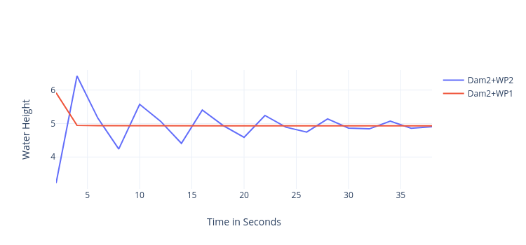
During the simulation, it becomes apparent that the height of the 1D wave propagation with dambreak2D start higher than those of the 2D wave propagation. The former reaches a steady state, while the latter exhibits a non-steady chart.
5.3. Personal Contribution
Ward Tammaa, Daniel Schicker Doxygen Documentation
Mohamad Khaled Minawe, Ward Tammaa, Daniel Schicker Sphnix Documentation
Daniel Schicker, Mohamad Khaled Minawe , Ward Tammaa functions implementation
Mohamad Khaled Minawe, Daniel Schicker, Ward Tammaa Unit Testing
Mohamad Khaled Minawe, Daniel Schicker Geogebra Datei(Calculations for the Unit Tests)
Ward Tammaa Hosting the code , Action runner